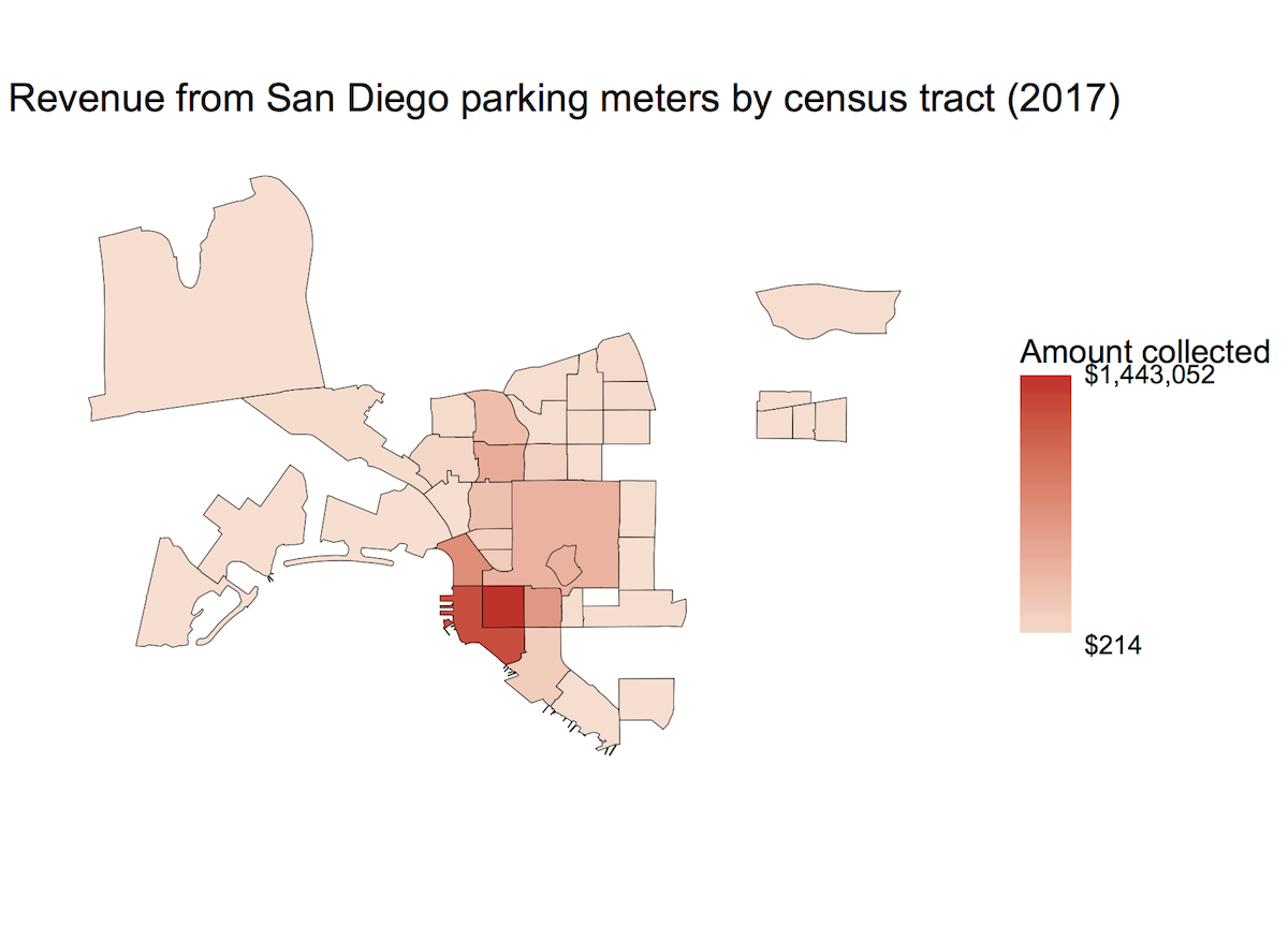
People Paid A Lot to Park Downtown This Year
Recently I’ve been working with a lot of GIS data, and I’ve been having a lot of fun making maps of the form “find the total value of some feature that can be attributed to all the things located in some region.”
The city of San Diego data portal has a lot of free data that I can use. This particular example is parking meter revenue by census tract. I get my census data from TIGER/Line.
I got the locations of the parking meters and the monthly revenue per meter from the City of San Diego. Next, I further grouped the parking meter data to be annual revenue (current as of yesterday). I cleaned up the data a little bit because there is a parking meter pretending to be in the ocean and some NA values and such.
To get the longitude-latitude information about the parking meters to play nice with the
shapefiles from the census, I needed to get them into a consistent coordinate system.
At that point, the over function was able to tell me which census tract each meter
was located in. And then I could group by census tract.
Finally, I converted everything to dataframes to plot with ggplot2. I also cropped the window to the uptown-downtown region of the city.
library(gpclib)
library(rgdal)
library(sp)
library(rgeos)
library(ggplot2)
library(scales)

# Parking meter data from City of San Diego
# https://data.sandiego.gov/datasets/parking-meters-locations/
# https://data.sandiego.gov/datasets/parking-meters-transactions/
# Download and save as meters.csv and transactions.csv in your working directory
# I manually took the spare meters out of the end of meters.csv
meters <- read.csv(file="meters.csv")
transactions <- read.csv(file="transactions.csv")

# Transactions for all of 2017
yr.transactions <- aggregate(sum_trans_amt ~ pole_id, data=transactions, FUN=sum)

# Converting from cents to dollars
yr.transactions$sum_trans_amt <- yr.transactions$sum_trans_amt / 100

# Combining locations with transaction totals
meters <- merge(meters, yr.transactions, by.x="pole", by.y="pole_id", all=TRUE)

# There is a meter with a bad value of longitude
meters <- meters[meters$longitude != -180,]

# Dropping rows with NAs
meters <- meters[complete.cases(meters),]

# Census tracts from... the census's TIGER/Line service
# Put the unzipped folder of shape files in your working directory
census.tracts <- readOGR(dsn="tl_2016_06_tract", layer="tl_2016_06_tract")

# Getting all the GIS data into the same spatial reference frame
coordinates(meters) <- ~ longitude + latitude
proj4string(meters) <- CRS("+proj=longlat")
meters <- spTransform(meters, proj4string(census.tracts))

# Which census tract is each meter in?
meters$tract <- over(meters, census.tracts)$GEOID

# What is the total value of sum_trans_amt added up in each tract?
the.values <- aggregate(sum_trans_amt ~ tract, data=meters, FUN=sum)

# We can also make a pretty picture with ggplot2
# Turn our GIS data into a dataframe and then merge (inner join)
census.tracts.fort <- fortify(census.tracts, region="GEOID")
the.values$tract <- as.character(the.values$tract)
my.geo.frame <- merge(census.tracts.fort, the.values, by.x="id", by.y="tract", all.x=FALSE, all.y=FALSE)
# Get all the vertices back in order
my.geo.frame <- my.geo.frame[order(my.geo.frame[,4]),]

# And now we can plot
ggplot(data=my.geo.frame, aes(x=long, y=lat)) + geom_map(map=my.geo.frame, aes(map_id=id, fill=sum_trans_amt), color="black", size=0.125) + scale_fill_continuous(low="#fee0d2", high="#de2d26", na.value="transparent", labels = scales::dollar_format("$"), breaks=c(min(my.geo.frame$sum_trans_amt), max(my.geo.frame$sum_trans_amt)), guide=guide_colorbar(title="Amount collected"))  + coord_map(xlim=c(-117.28, -117.05), ylim=c(32.67, 32.81)) + theme_void() + ggtitle("Revenue from San Diego parking meters by census tract (2017)")